In Baron & Poznanski (2016) we find the most spectroscopically peculiar galaxies in the 12th data release of the Sloan Digital Sky Survey (SDSS). There, we describe in detail the algorithm that we developed, calculate the 'weirdness' of about 2.5M galaxies, and discuss the weirdest 400.
A brief explanation of the outlier detection algorithm
Our purpose is to rank objects by how different they are from all the others. For this, one needs to compute some distance matrix that contains the distances between every pair of objects in some (non-euclidean) space. We compute this matrix using Random Forest (RF). The objects that are farthest from all the others are the biggest outliers. We simply look at the objects with the largest average distance from the others.
How RF is typically used
In supervised learning, RF is used to classify objects for which there exists a training set of labeled objects (i.e., we know the class of these objects). The RF then aims to learn how the features (the properties of the objects) can point to the correct label. RF does that by creating many decision trees. In any such tree, a random subset of the objects, and a random subset of the features is selected. Then, the algorithm finds the value of a given feature that divides the sample best. Then, every branch is further split to maximize separation between the classes. After a few (predetermined) such splits, the end nodes of a tree - the leaves - should each contain mostly objects that belong to one of the classes. Having generated many such trees, the RF can now, given a new object of an unknown class, pass it through all the trees, assign a class by majority vote.
Unsupervised RF
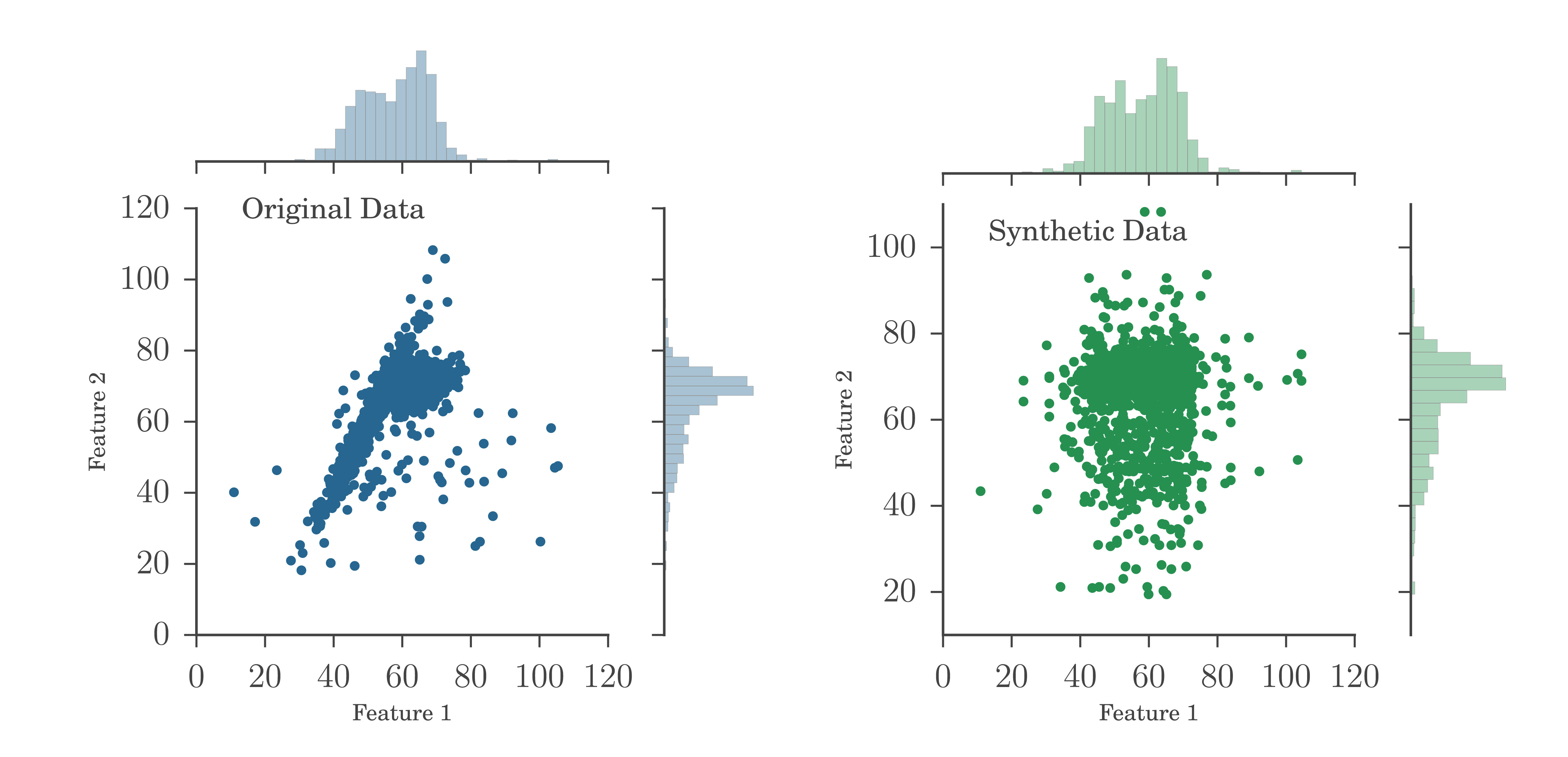
For the problem of finding outliers we do not have a training set. Instead we take our entire dataset - label it as class "real", and generate a synthetic dataset of similar size, and similar marginal distributions in all the features, but without covariance between the features (see example in the figure below). This dataset is labeled "synthetic". We therefore have now two classes in our training set, with the only difference between them being the existence or lack of covariance. Training the RF on these sets teaches it to recognize objects that have covariance. Now, given two objects that we pass through all the trees, we can ask how often they ended up in the same "real" terminal leaf. Two completely identical objects will have the exact same features and always end up together. Two very dissimilar objects will never do. Therefore, counting how often two objects land in the same leaf is a measure of similarity, or distance, which was our purpose.
Some additional thoughts
The algorithm performed very well on galaxy spectra, where the features were simply the fluxes at every wavelength. We define "very well" in that it found interesting outliers of different kinds. A galaxy that is similar to many others, except for, say, emission lines that are all stronger, is less interesting to us (as astrophysicists, this is not a mathematical definition) than a galaxy that shows unusual ratios between some lines, which points to different physical settings (radiation field, ionization, etc.). Since we trained our machine to identify covariances, to separate "real" from "synthetic", it finds exactly that. Basically, most of the physics in a spectrum is in the covariance (and higher order moments). Line width can be seen as a covariance on short scales, the continuum is covariance on large scales, and line ratios are covariances between specific wavelengths. This likely extends to other types of data, images for example, and we would love to hear your experience using our algorithm for your purpose.